Weather predictions from satellite data
You have now received weather satellites, such as NOAA 15, METEOR-M, and the like. The images are pretty and nice, but after a while it gets boring. However, these are weather satellites. Wouldn't it be cool to learn how to predict the weather with the data you receive?
You've come to the right place!
WARNING The contents of this page are still under development, so be sure to come back frequently for updates (last update
January 4, 2024). Additionally, the contents of this page are NOT to be used for operational meteorology but only at the hobbyist's level!
The beginning
In order to use weather satellites, you have to first understand how the weather works, and what patterns to look for in the satellite imagery.
How weather works
The Sun's energy is the driving force behind basically all weather phenomena on Earth. Its energy heats up the seas and ocean, making water evaporate. Water vapor then is pushed by winds (also caused by the Sun) and finally condenses in the colder, upper layers of the atmosphere, where it turns into rain.
Does this ring a bell? Of course it does, it's the water cycle!
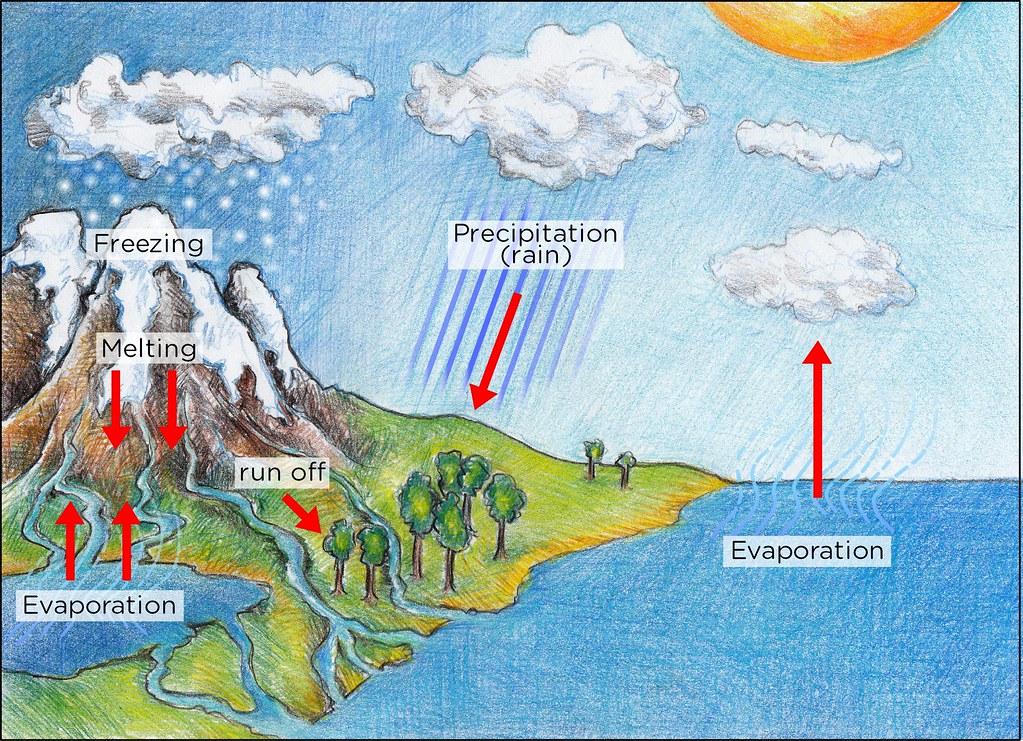
Credit: Siyavula Education
Look at the clouds!
The first thing you need to do is know your clouds. Learn them, and learn to recognize them both in satellite imagery as well as using your Mk.1 eyeballs.
To an untrained eye, all clouds look similar, although some do look more menacing than others. Have you ever noticed clouds similar to these?
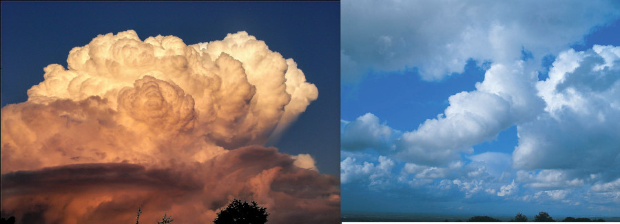
Credit: Brigitte Alliot, Thennicke
The first cloud does look quite scary, and rightly so! It even has a name: cumulonimbus. It is usually associated with thunderstorms. But what about the second one? It looks less menacing, but are we sure?
Well, the second one is a cumulus. It's a fair weather cloud, it doesn't usually do harm unless you're sunbathing. But, feed it a bit too much water vapor and it gets fat, so fat it almost reaches the stratosphere, which means it will be very cold. Now, it becomes a cumulonimbus. The taller it is, the colder it will be, and the stronger the chance of a thunderstorm.
Cloud classification
To make our life easier, we meteorologists have classified clouds, and given them some names and a two letter identification code. Here are the most important ones:

Credit: Valentine de Bruyn
Here is a good resource to learn more about cloud classification.
Classifying clouds on the satellite
Classifying clouds with your eyes is easy, because you have a three-dimensional view of them! Just by looking up the sky, you can see where the top is, the shape of the cloud, how dark it is, and how tall it is relative to the ground.
You don't have this luxury on the satellite, because it takes a bird's eye view on the cloud. You cannot see the bottom, and you lose depth perception.
For example, take this example image. How would you classify each cloud?
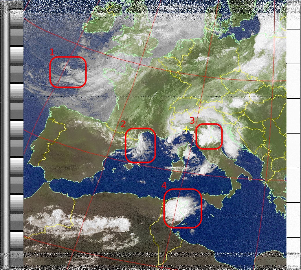
NOAA 15 2023-06-30 18:31 UTC
How does a satellite «see»?
Usually, people think about weather observation satellites as a camera on a satellite. While in very broad terms this is true, it's also not so easy...
Weather satellites use radiometers to «see». These instruments scan the Earth line by line, instead of taking separate pictures at regular intervals.
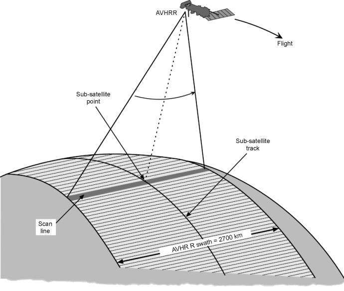
© adapted from Minnett (2001)
Furthermore, satellites do not see like our own eyes, or a camera. A camera sees all light that has a wavelength between about 380 and 750nm, or between violet and red.
The AVHRR and MSU-MR radiometers on the other hand see only distinct frequency bands, called channels, and not an entire spectrum.
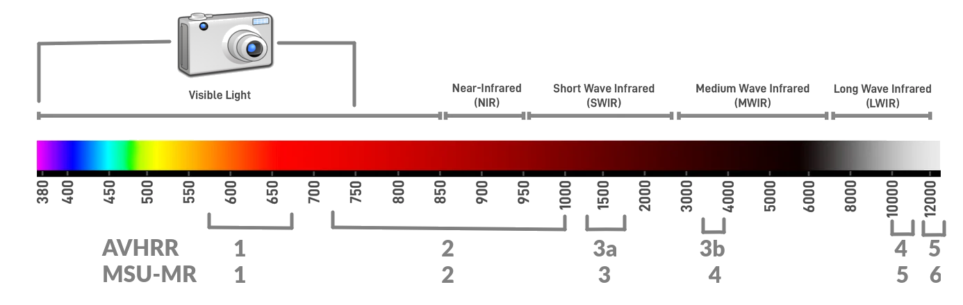
© Clearview, used with permission. The scale is in nanometers.
As can be seen, except channel 1, all other channels are in the infrared region, and for a good reason! The world «looks» different when observed in the infrared range, and what is difficult to see with our own eyes, can stand out much more in the infrared range!
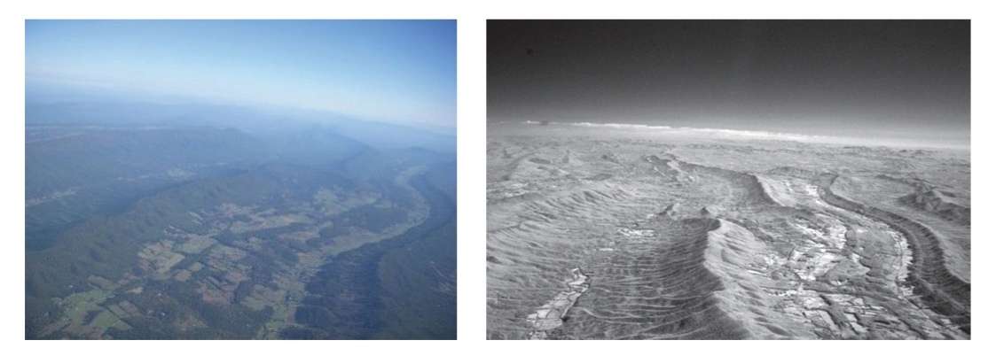
© adapted from Campbell et al (2022). Difference beetween a visible photograph and the same scene taken in the near-infrared range.
Each channel on the radiometer has a purpose.
| Center wavelength | AVHRR | MSU-MR | Usage |
|---|---|---|---|
| 0.630 µm | 1 | 1 | Cloud classification, vegetation, land usage |
| 0.862 µm | 2 | 2 | Cloud classification, vegetation (chlorophyll) |
| 1.61 µm | 3a | 3 | Snow and ice detection |
| 3.74 µm | 3b | 4 | Cloud classification at night, fire detection |
| 10.8 µm | 4 | 5 | Cloud top temperature, temperature measurements |
| 12 µm | 5 | 6 | Cloud top temperature, convective systems analysis, ash detection |
The ability of the radiometer to «see» in the far infrared bands (thermal infrared and longwave infrared) makes it possible to observe the Earth at night, as well as to measure temperatures. This is very important.
Making your life easier
If you looked closely at the cloud classification diagram, you might have noticed that different clouds have tops at different altitudes. Higher altitudes mean colder and colder temperatures.
So, how do we interpret temperature from the satellite? Well, we could just look at how "white" the cloud is (whiter means colder, in satellite imagery).
However, we quickly find that our eyes cannot really see more than 5-6 shades of gray, while the satellite uses 256 of them! Fortunately, our eyes are capable of also recognising colors, so we can turn the image into a false color one. That process is called using a LUT (Look Up Table). It's essentially a table that associates a temperature value to a specific color, like -73°C means red.
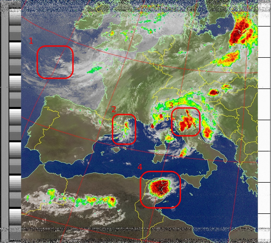
NOAA 15 2023-06-30 18:31 UTC
Now it's fairly easy to classify this image:
- Altostratus clouds
- Stratocumulus clouds
- Nimbostratus clouds
- Cumulonimbus cloud
Seeing where the clouds go
So, you have recognized your cloud types and now see something like this. How do you know it's not heading towards your house?
Coriolis effect and prevailing winds
First things first, there is a pattern to storm movements. They tend to come from the West and go to the East.
Then another thing can help you with that kind of small storms, the tail. Prevailing winds will tend to "blow" the cloud away like it's some sort of candle flame, and the tail will tell you the prevailing wind and therefore which direction it will go.

How can you be sure?
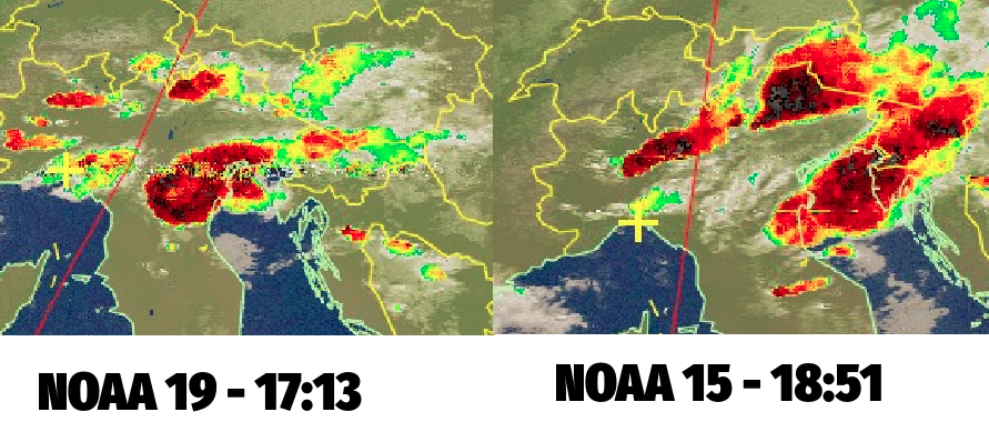
Well, for that you need several satellite passes, and that's the reason why satellites are divided in AM and PM orbits. In the POES system, you have NOAA 15 (backup) and 19 (prime) in the AM orbit, NOAA 18 (backup, the prime being NOAA 20) in the PM orbit.
So, if you get a NOAA 15 and then a NOAA 18, you can see how much the storm has moved
You can also use a NOAA 15 and a NOAA 19, and this provides a separation that depends on their orbit but can go as long as almost 2 hours.
For further details on cloud classification via satellite observations I recommend reading Cloud Investigation by Satellite by Richard Scorer (Ellis Horwood, 1986)
Atmospheric pressure
The weather is closely related to atmospheric pressure. We've all heard the term depression or cyclone, as well as anticyclone. But what do those mean, and how can we use those to forecast the weather?
High pressure (anticyclone)
A high pressure area, as the name implies is an area where the atmospheric pressure is greater than the surrounding areas.
This means that air will be "pushed out" from the center (where the pressure is highest) to the periphery and to lower pressure areas.
The incresed pressure will dry out the atmosphere resulting in usually clear skies and fair weather, the opposite of a cyclone (hence the name). Therefore, it is usually easy to determine the location of a high pressure area from satellite imagery as there will be a "hole" in the cloud cover, with neighboring clouds being "pushed out" by the difference in pressure.
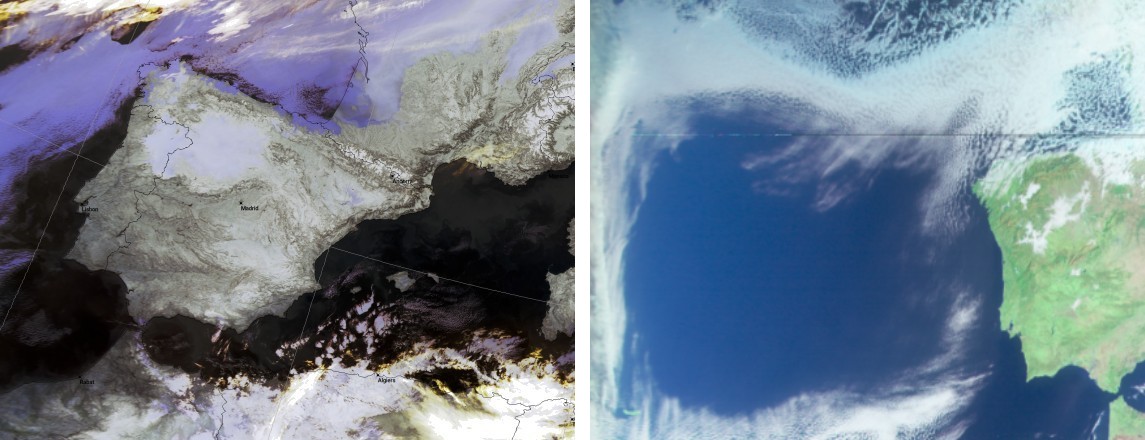 Left: A high pressure area over Spain and Western Europe as seen by Metop-B. You can see the pressure difference preventing the clouds over the bay of Biscay from advancing.
Right: Another anticyclone over the Atlantic as seen by Meteor-M N°2-3, showing the characteristic "hole" in cloud cover. Image kindly provided by 2M0IIG.
Low pressure (cyclone)
A low pressure area conversely is an area where the atmospheric pressure is lower than the surroundings. These areas are associated with inclement weather (think hurricanes).
They have a peculiar spiral shape that spins in different directions depending on the hemisphere:
- clockwise in the Southern hemisphere (Australia, South America...)
- counterclockwise in the Northern hemisphere (Europe, most of Asia, North America...)
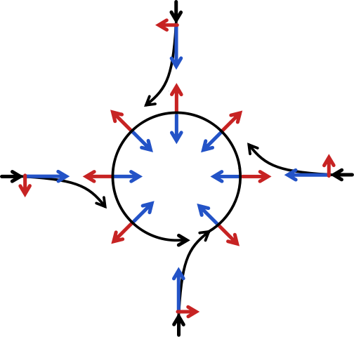
This diagram shows the wind circulation (in black) in a Northern hemisphere low pressure area. Red arrows show the Coriolis effect induced forces and the blue arrows show the pressure difference induced forces. © Roland Geider, used with permission.
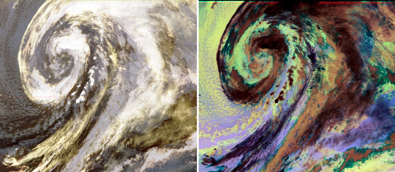 An excellent capture of a cyclone over the Atlantic by NOAA 19 both in infrared as well as microphysics.
It is important to note that it will not always be possible to see the entire spiral as in the image above, as these structures can sometimes be very large, often exceeding the swath shown by the satellite. You'll often see only part of the system.
Tropical cyclones
Additionally, if the low pressure system forms in the tropical zone, the system can develop in a tropical cyclone. This is one of the most powerful weather phenomena on Earth.
A special method and algorithm was developed by Vernon Dvorak between 1969 and 1984, and therefore is referred as the Dvorak method. Hurricanes tend to develop in distinct patterns, and these patterns can be used to predict the strength and duration of the hurricane according to the Dvorak method.
The table below shows different developmental patterns of hurricanes and their Dvorak numbers.
The BD enhancement is used to enhance particular temperatures that are common precursors (this will be explained later).
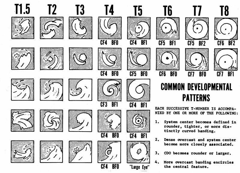
© from Dvorak 1984
Fronts
What are weather fronts (shortened to just fronts), and how are they related to weather forecasting?
Fronts are basically borders separating air masses that have different characteristics. As these air masses mix together at the front, unstable weather can occur along the front.
This instability can bring thunderstorm, rain showers as well as cyclonic activity and very strong winds: it is for this reason that it is very important to study them and learn to recognize their shape on the satellite imagery.

Different fronts. The symbols point towards the direction of travel.
Cold front
As the name suggest, the cold front is the leading edge of a cold mass of air, that replaces a warmer mass of air. It often forms behind (East in the Southern Hemisphere, West in the Northern Hemisphere) an extratropical cyclone.
Along the edge, thunderstorms or rain can occur, depending on the instability of the front (more unstable fronts tend to bring stronger thunderstorms).
On the satellite, it can be recognized by clouds in a straight line.
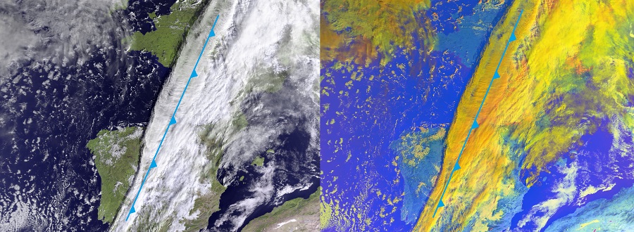
A cold front over Western Europe as seen by Metop B, in both natural color as well as day microphysics.
Squall lines and derechos
A squall line is part of a cold front and usually occurs during the summer months when the air is hotter and more turbulent. It consists of essentially very strong thunderstorms along the line.
A squall line can further evolve into a derecho, a very strong phenomenon that is both large in size (often 500km in length or more) and with extreme characteristics, such as a sustained wind speed of over 90 km/h.
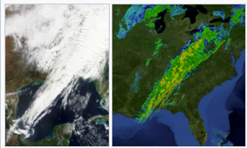
A squall line over the Eastern United States as seen by the GOES-R satellite. © NOAA
Warm front
A warm front is the leading edge of a warmer mass of air. Compared to cold fronts, they move slower and are usually followed by them.
Clouds at the leading edge are usually nimbustratus, rarely cumulonimbus. Rain is usually moderate but persistent until the front passes.
Warm fronts can also bring snow, if the temperature at the ground is cold enough.
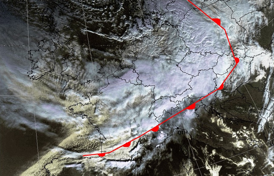
A warm front over most of Europe as seen by NOAA 18.
Occluded front
An occluded front can form when a cold front overtakes a warm front, near a low pressure area. To determine if a front if occluded, find a low pressure area and check if there is a tell-tale split between the clouds.
There are two types of front occlusions:
- A cold occlusion, where the cold air mass that overtakes the warm air mass ahead is colder than the cool air at the very front and plows under both air masses.
- A warm occlusion where the cool air mass overtaking the warm front is warmer than the cold air ahead of the warm air mass and rides over the colder air mass while lifting the warm air.
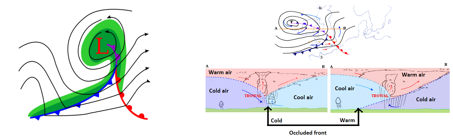
© Ravedave, used with permission.
Precipitation
Precipitation occurs when specific patterns arise in the atmosphere
Dynamic (stratiform) precipitation
As discussed above, fronts tend to cause precipitation of different characteristics depending on the type of front.
Cold fronts bring very intense rain showers and thunderstorms, while warm fronts tend to bring persistent but moderate precipitation.
Convective precipitation
As hotter, more humid air is lighter than cold air, it rises up. When it gets cold enough, it will condense and precipitate.
Convective precipitation tends to produce short rain showers lasting no longer than an hour, but can be very violent especially in the tropical areas.
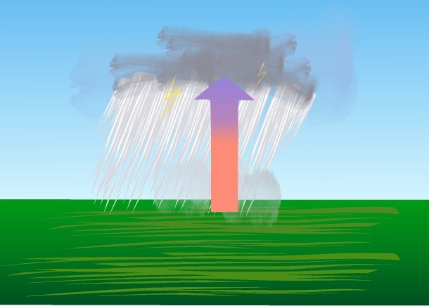
© Severin Heiniger, used with permission.
Orographic precipitation
If the ground they touch has a mountain range on the path of the storm, it will force the cloud to go up, which will make it hit colder layers of air, and therefore condense more easily into rain. If the storm is constrained between open sea/ocean and a mountain range, the rain can be very intense, while the other side of the mountain range usually gets little to no rain. This is the case in Hawaii as well as in the Andes, Himalayas, Appennines and Sierra Nevada.
However, while the values for such rainfalls might be extreme (even over 1000 mm/h), the hydrographic features (rivers, lakes) of the areas where this occurs are usually adapted to cope.
For example, Liguria in Italy is a region where these phenomena are very common. Rains of over 950 mm/h have been recorded (Rossiglione, November 2022) with no flooding occurring.
Conversely, in nearby Toscana, 600 mm/h of rain was enough to cause severe flooding in November 2023.
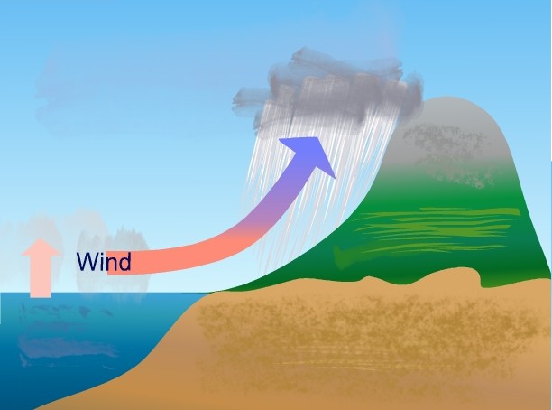
© Severin Heiniger, used with permission.
Atmospheric temperature profile
We've talked extensively about how clouds rising get colder, how the cloud height directly determines the strength of a storm, and how it is useful to determine the temperature of a cloud top using the radiometer. In order to find the cloud height in meters from the temperature, we can use the standard atmospheric curve.
© Loic Jounot. 1976 US Standard Atmosphere temperature curve.
As far as meteorology goes, we are only interested in the lower part of the curve, labeled as Troposphere. This part is linear, and has a gradient of approximately -6,5 °C per km.
It goes without saying that this is true only for a dry, undisturbed atmosphere! Water vapor will alter this temperature gradient. However, despite this, we can still use the gradient with some approximation to our advantage, and especially the tropopause is extremely important for our purposes as it serves as a "ceiling" to storms. This will become evident later in this read.
How do storm forms?
Sea
The open sea is a good breeding ground for storms as it is where the water vapor of the actual rain comes from. High water temperatures of 26°C or more cause an increased chance of very strong storms or hurricanes especially in the Mediterranean and similar mid-latitudes.
Recognizing the beginning of a thunderstorm
A storm will not immediately appear from nowhere. Storm development takes at least a few hours, as it goes without saying that a storm cannot occur if there are no clouds in the area!
The development cycle of a thunderstorm at mid latitudes usually begins over the sea or a large lake. Clouds develop into cumulus, then as they rise progressively they turn into cumulonimbus and finally dissipate.
The arrows in the diagram indicate convection.
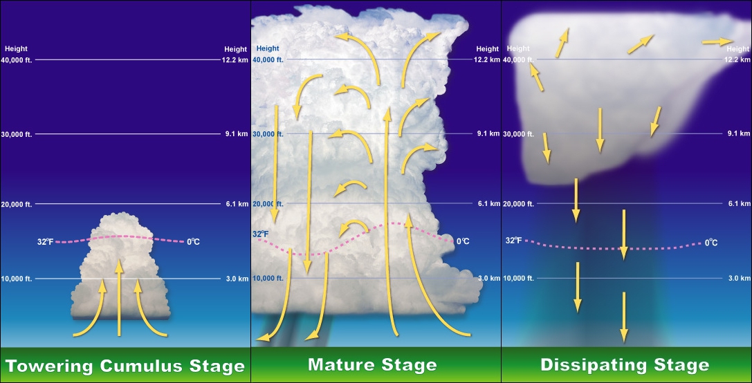
© NOAA
BEWARE: Tropical areas behave differently due to the much greater heating from sunlight. Therefore, convective systems develop much more rapidly, often in a matter of an hour or less, and the resulting precipitation is often extreme.
Computer-assisted imagery analysis
Now you've seen the basics, can track the clouds, and you can also try recognizing a brewing storm. You can still analyze your images by hand "just like in the old days", but even in the 1960s there were some enhancements developed to make the meteorologist's life easier by using computers to do much of the heavy lifting, assisting the meteorologist in its work.
Traditional enhancements
These enhancements were originally designed in the early era of weather satellites are almost all in black and white. They all take infrared data from the thermal IR channel (10.8 µm, channel 4), except the Color convection longwave IR enhancement which uses longwave IR (12 µm).
All but Color convection longwave IR work on both APT and HRPT data.
The list includes MB, CC, EC, HE, HF, MD, BD, NO, ZA, TA, JF, JJ, Cloud general cloud IR, Enhanced IR and Color convection longwave IR.
Extensive documentation is available in SatDump by selecting the enhancement and clicking on the ⓘ Info button.
For a quick look at the current situation, the
Enhanced IRorNO(cloud top temperature measurements), andColor convection longwave IR(convection structures detection and analysis) are usually used.
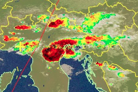
 The MD enhancement in use on NOAA 15, showing a mid-latitude cyclone over the Gulf of Genova.
Advanced enhancements and composite imagery
APT and optical observation is enough for basic predictions and it will get you very far.
In fact, I might owe my life to NOAA 15, as it provided me with very up to date information about one of the worst storms ever to occur in the Mediterranean, just as I was sailing right into it and, being in the middle of the sea on my boat, had no cell service or radio reception.
For more advanced stuff and more precise forecasts, having more than 2 channels (3 on LRPT) enables you to use several more tools, in addition to applying the same principles as above but with greater precision due to the higher resolution.
Additionally, data from other sensors can be overlaid on top.
Advanced enhancements
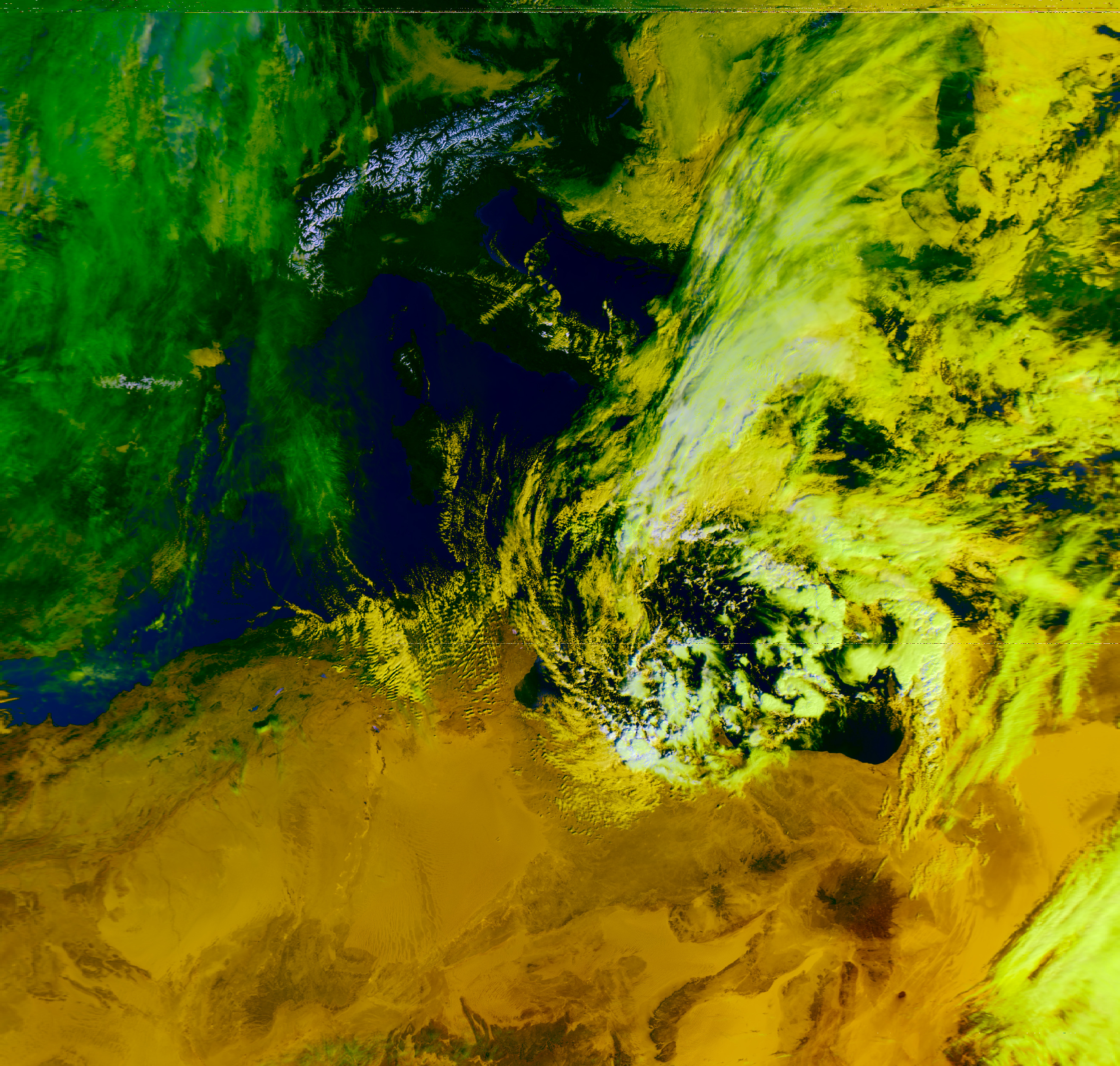
Microphysics
As we have seen it might sometimes be hard to differentiate between fog and low clouds, or between water vapor clouds and clouds that are just starting to ice up. This is where the microphysics enhancements come into play, and there are two variants of them: Day microphysics, and Night microphysics.
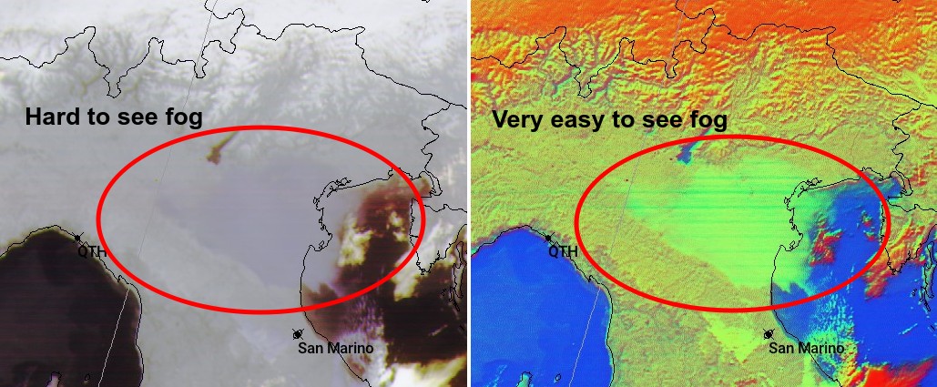
The interest of microphysics is better determination of phenomena that can have low contrast.
A detailed explanation for both can be found in SatDump by selecting the enhancement and clicking on the ⓘ Info button.
124
(125 on Meteor-M)
This is an enhancement that blends channel 4 or 5 (thermal IR) with visible channels 1 and 2. This enables you to see cloud shadows and see the terminator better.
Additional information can be obtained in SatDump by selecting the enhancement and clicking on the ⓘ Info button.
Snow (Metop HRPT only)
By making use of the channel 3a, snow cover can be enhanced and differentiated from white clouds.
Additional information can be obtained in SatDump by selecting the enhancement and clicking on the ⓘ Info button.
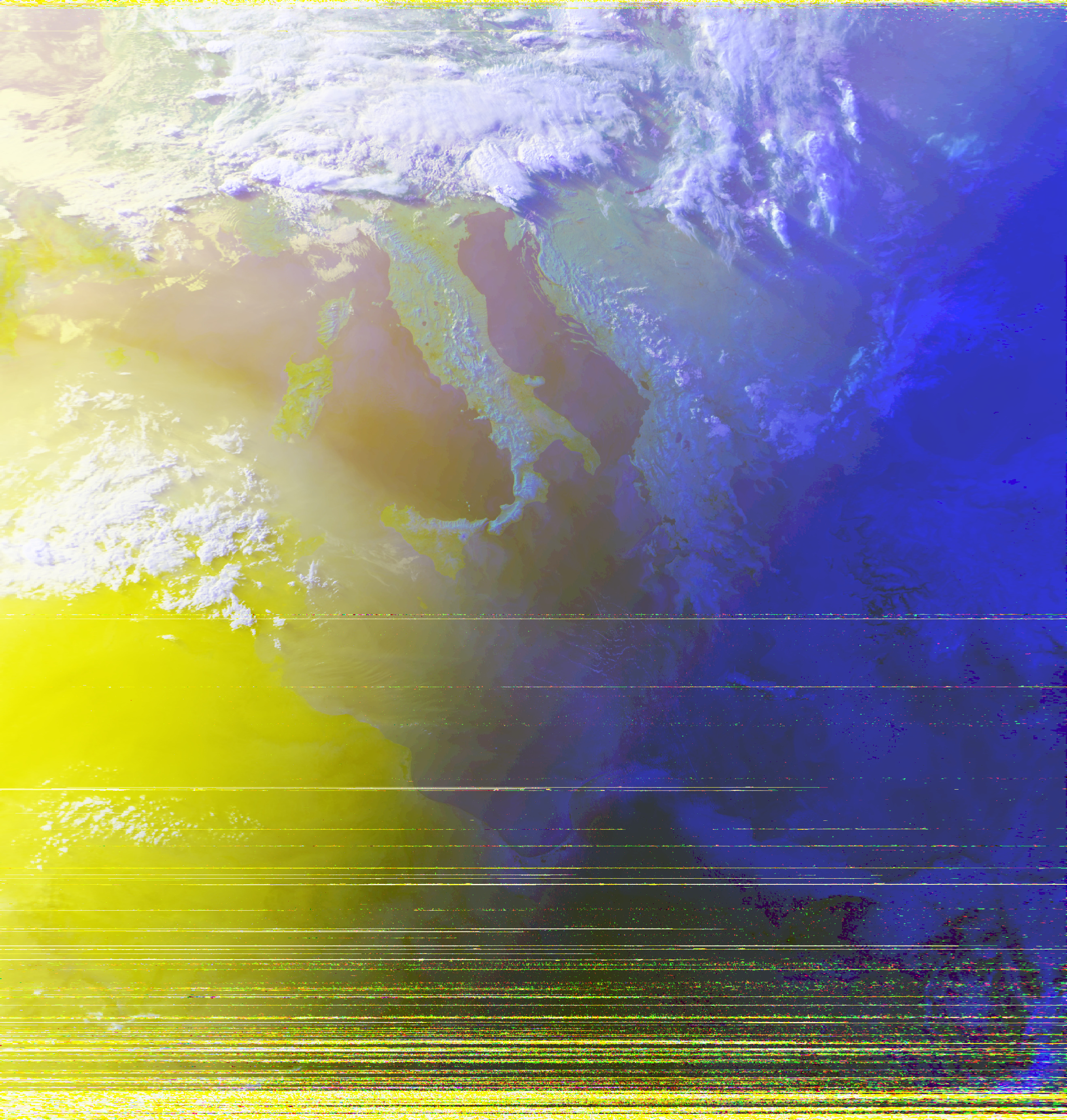
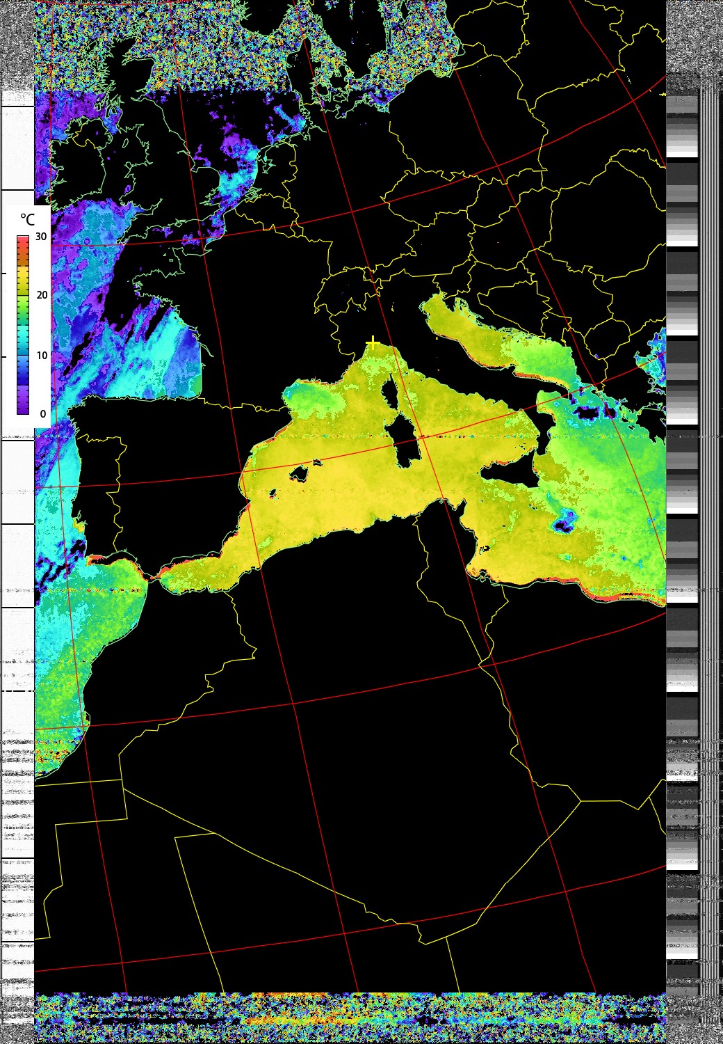
SST - Sea surface temperature
It is essentially a LUT tailored to the range of temperatures expected to be found on a sea, made from the difference of 2 IR channels (5 and 4 on NOAA/METOP, 6 and 5 on Meteor-M), with a correction factor and with a land mask that will completely cover the ground.
Additional information can be obtained in SatDump by selecting the enhancement and clicking on the ⓘ Info button.
Caveats & warnings
Nothing would be complete without some caveats, so here are some.
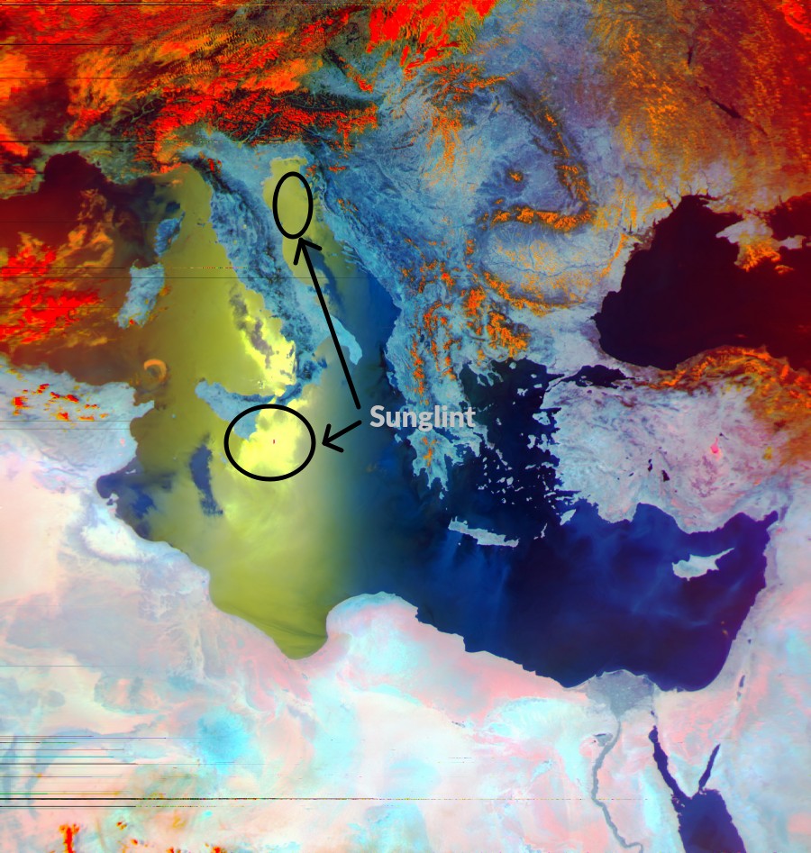
Sunglint
On satellites that are at an AM orbit (Meteor-M N°2-3, NOAA 15, NOAA 19, Metop B) or a late PM orbit (Meteor-M N°2-2) the reflection from the sea (called sunglint) will "blind" the radiometer in the visible channels, making it hard to interpret what is in there
Seasonal variations
Of course the range of temperatures acceptable for the sea varies with the seasons. The night microphysics also is sensitive to seasonal variations. The MB thunderstorm enhancement should only be used in winter, and the MD enhancement should be used instead in the summer or in warmer climates.
Interference from thin clouds
Purely thermal measurements, such as SST, will be skewed by thin clouds, fog or haze, so always check with microphysics if that's the case if you see unusually low sea temperatures (also see the next item).
Bad calibration
As satellites age, it is necessary to compensate the alterations in the detectors inside the radiometer by the way of calibration curves. Satdump usually deals with this automatically (unless there are bugs), but other software might not especially Wxtoimg. Therefore, if you see unusual temperatures, or too bright/too dim clouds, it might be a calibration issue. In that case double check with another satellite pass, after checking there was no haze/cloud in the way.
No calibration
Roscosmos/Roshydromet has yet to publish calibration curves for the MSU-MR in the Meteor-M N2-3, therefore Meteor satellites are not calibrated and can only be used for qualitative measurements.
Additionally, even for satellites where the calibration curves have been published, the software in use might not do calibration compensation. For APT, only SatDump and Wxtoimg support calibration.
Sounders
You are now able to predict the weather with a fairly good accuracy but there are still some limitations, namely:
- You can only guess if it is raining, not actually know
- You can only guess how much water the cloud is holding
- You can't see different layers in the atmosphere
- You can't take temperature measurements if there is a cloud on top.
Enter sounders, a variety of instruments designed to perform several different measurements, both into and below the clouds.
MHS (Microwave Humidity Sounder)
This is the newest instrument we'll be talking about for now, as it has been developed to replace the AMSU-B on NOAA 18. It is currently operating on NOAA 19, Metop B and (with limitations) on Metop C.
It works by detecting not visible light, but rather radio waves.
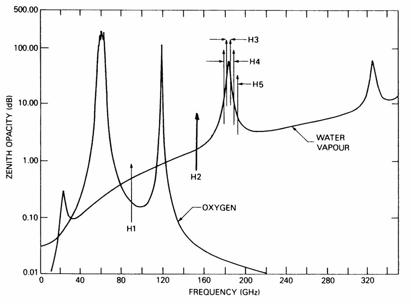
The atmosphere has several absorption bands in the radio spectrum, that can be utilized by the sounders to measure things like water vapor content, rainfall rate, total cloud liquid water content, etc.
Here's a graph showing the relation between frequency and absorption ,as well as the different channels used by the MHS.
Products
Additional information can be obtained in SatDump by selecting the enhancement and clicking on the ⓘ Info button.
221
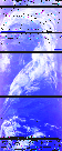
The easiest composite you can get out of MHS is called 221, as it puts channel 2 in both the red and green parts (making it appear yellow), and channel 1 in the blue. The channels H1 at 89.0GHz and H2 (157GHz) are window channels (not affected by clouds). H1 detect water vapour in the very lowest layers of the atmosphere and rain, whereas H2 is a pure window channel.
Interpretation: Black indicates that precipitation is occurring, progressively lighter shades indicate progressively less water content in the clouds at low altitude, usually below 1km, very light shades of blue are artifacts and should be ignored
WARNING It will get fooled by snow easily in the winter.
It is always better to use it in conjunction with an imaging radiometer, as there are many caveats when using such simple enhancements.
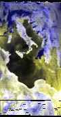
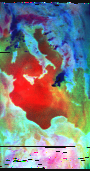
In the image below, you see a lot of blue. But what is rain, and what is snow? You could guess that snow can't be in Greece, so it must be rain. But what about on the Alps?
421
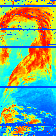
This composite connects the MHS channel H4 to the red channel, MHS channel H2 to the green channel, and MHS channel H1 to the blue channel.
H1 provides detection of water vapor, H2 provides a window channel for the geography and H4 makes snow stand out in a different color.
This composite is better than 221 as it will render water vapor clouds in different shades of blue, snow in pink/magenta, and the geography in various shades of green or red, but it still can't detect actual rain (like rain that is happening right now) in an unambiguous way.
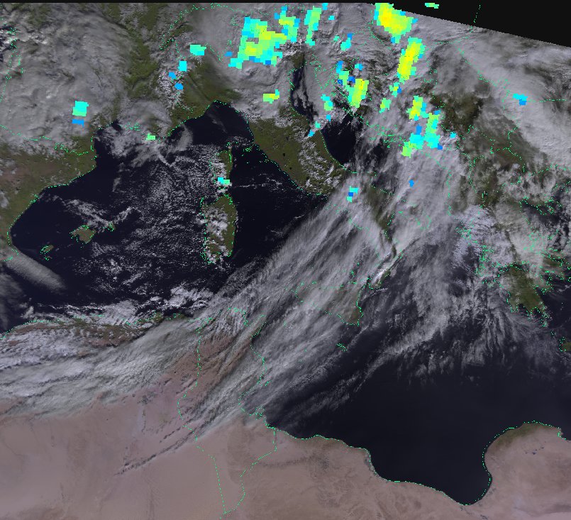
Rain
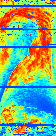
This is a perfect algorithm to detect exactly where rain is happening right when the satellite is passing. The principle of operation is really easy: transparent = no rain, red = lots of rain, shades in between = different quantities of rain.
It works best when overlaid on top of either a map or an image from the radiometer:
Snow
The MHS can also detect and quantify snow cover on the ground.
Significant thunderstorm cells
The MHS can detect thunderstorm cells by measuring the inner cloud temperature.
How to interpret rainfall data
If you see a storm approaching, you can track the rainfall and be able to predict with great precision what the storm is doing by just watching the rate of rainfall. For instance, when the storm finds a mountain range in its way, you will see the rainfall rate increase. When the storm is dissipating, you will immediately see the rainfall rate decrease.
Special case: If, by using the other enhancements given by the main radiometer, you still see a lingering cumulonimbus, but no rain, it might very well be a self-regenerating storm cell. These cells are more and more common as global warming progresses and are usually found in coastal areas near seas. The rain will cease for a while before another cold current makes it precipitate again. These storms can be devastating and one of them caused the 2011 flood in Genova, Italy which devastated the city.
HIRS and IASI
The HIRS is one of the most useful instruments flown on POES satellites, however its potential has never been realized due to the lack of work decoding it and especially developing composites and enhancements for it.
This sounder is also the only one you can get if you don't do HRPT (or can't) making it very easy to get and extremely useful, especially since you can easily do it on the go. It is broadcast on DSB (as well as HRPT, of course) at 137.35 MHz for NOAA 15 and 18, and 137.77 MHz for NOAA 19.
The way HIRS work is simple: imagine taking AVHRR, giving it 20 channels instead of 6, reducing the resolution but enhancing the precision.
The channels (bands) are carefully chosen so they can be used to measure very specific atmospheric phenomenons.
For example, HIRS uses CO2 absorption bands for temperature sounding at specific altitudes (CO2 is uniformly mixed in the atmosphere). HIRS also measures water vapour in several different layers of the atmosphere, ozone, N2O content, cloud and surface temperatures. HIRS can be used effectively to detect haze and thin clouds that are not easily detectable on AVHRR, especially at night.
Metop satellites up to Metop B have flown both HIRS and a new development called IASI. IASI is essentially a SDR for infrared light, it has a channel for every wavelength in a specified range. Therefore, it can also do what HIRS does and is therefore equivalent to HIRS as far as meteorology goes.
Useful Products
Cloud only
This was my first composite I developed for HIRS, and I remember fondly the response of one of the authors of SatDump (Zbychu): "Finally we have an use for HIRS!"
Making use of the N2O absorption channels 14 and 13, it enhances the clouds over a blue background, the clouds appearing progressively whiter as their thickness increases.
Water Vapor
This enhancement enables you to see water vapor content in two different layers of the troposphere (The lower part of the atmosphere). This enables you to track cloud height. It makes use of the 9.71 µm channel for low level and 7.33 µm for the medium level.
The water vapor can help you predict where clouds could form, together with the next item.
Tropospheric and Stratospheric Temperature
Thanks to the channels that are CO2 absorption bands, it is possible to precisely measure the temperature at different layers of the atmosphere, giving an unique view of the layers constituting the atmosphere like if you were doing balloon (radiosonde) soundings, and enabling you to see a 3D representation of the atmosphere as temperature goes. This is WIP will be completed in the near future when HIRS is calibrated.
Blending with optical imagery
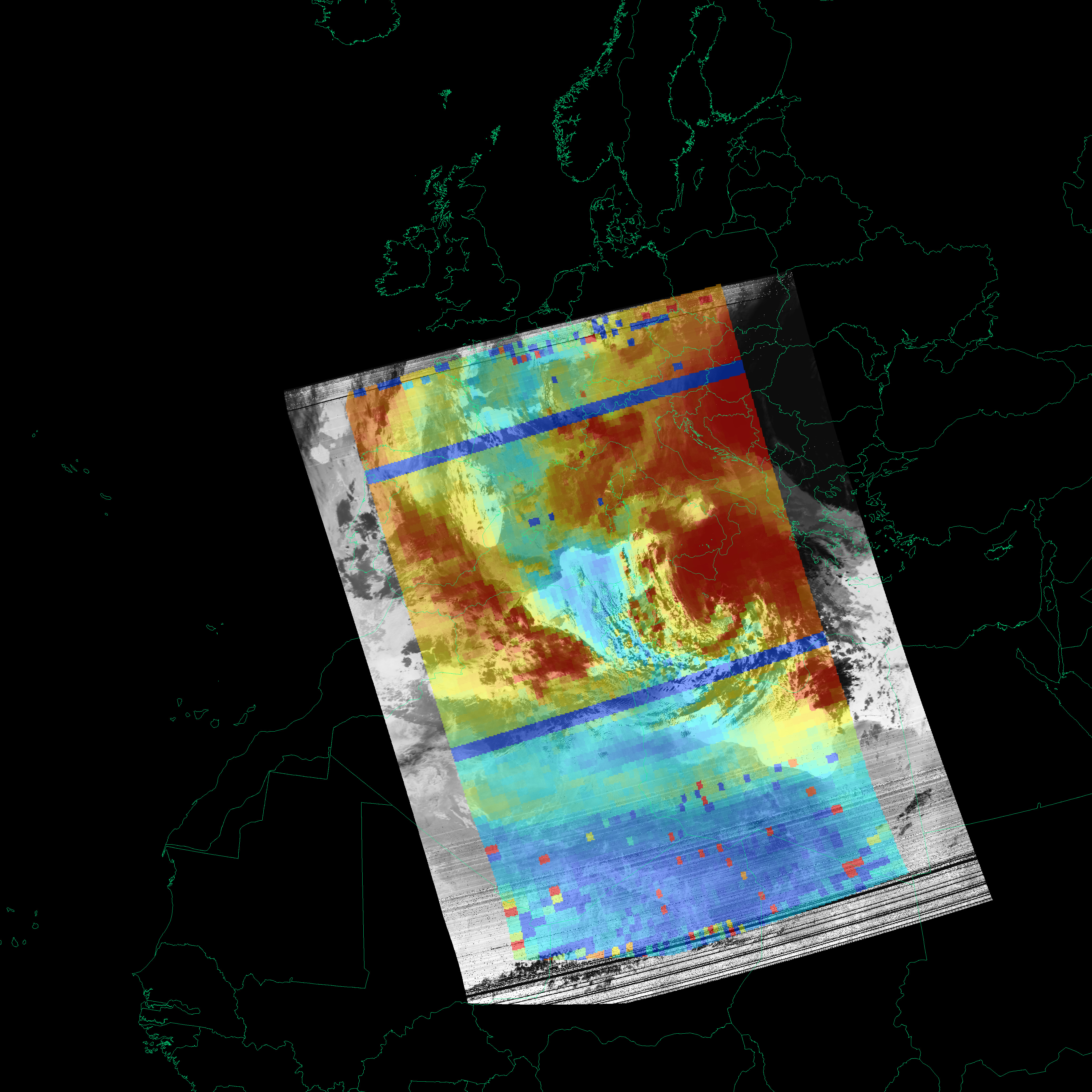
As with all sounders it is very useful to blend in images from an optical radiometer such as AVHRR; in order to better understand the situation. Here's high level water vapor blended with AVHRR thermal channel.
Advanced Microwave Sounding Unit (AMSU)
The AMSU is another microwave passive sounder, a lower-resolution MHS with more channels if you will. Its main purpose is to get very precise temperature measurements at the surface or in specific layers, even when there are clouds, using the oxygen absorption principle.
The AMSU as the name implies is an advanced version of the MSU, an instrument flown on all NOAA satellites since TIROS-N (1979). Data from the MSU (and AMSU) has been crucial in tracking global warming, and is actually from the MSU temperature soundings that the graph of warming Earth you are all familiar with has been derived, as it provides full globe coverage.
As you can see in the graph below, MHS and AMSU are very similar instruments, operating on the same principle. In fact, before the European-designed MHS was deployed on NOAA 18, NOAA satellites used two AMSUs - AMSU-A and AMSU-B, which had similar channels to MHS.
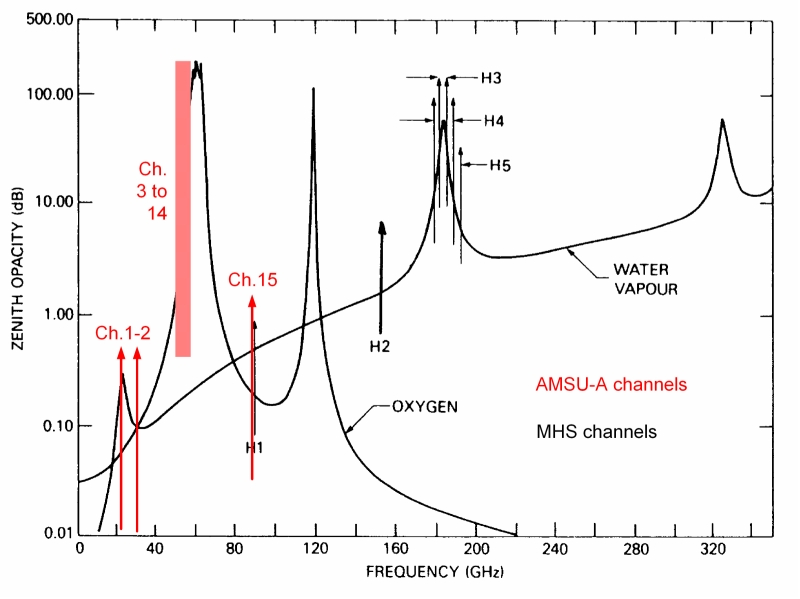
Now, how could this data be utilized? Remember the vertical temperature profile of the atmosphere? Now, let's put it against a graph that shows the sensitivity of each AMSU channel to different altitudes:
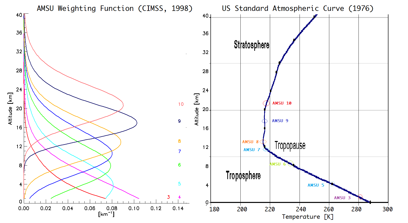
AMSU weighting functions (by CIMSS, 1998) vs US Standard Atmosphere (1976) with altitudes shown. Altitudes will depend on atmospheric pressure, but won't be altered by water vapor or clouds.
This is a huge capability and can allow us to determine with great precision the cloud top height, or the extent to which a storm is developed (remember, greater height = stronger storm).
NOAA 18's AMSU channel 8 (15 km altitude, 100 hPa pressure) shows a hot anomaly caused by typhoon Neguri, in 2014. © CIMSS.
Useful Composites
543
This is designed to be a composite that is easy to use and look at. It provides a false color, cloud less view differentiating between sea (appears blue-red), land (appears blue-violet) and snow/ice (appears black).

Pressure temperature
These composites show the temperature at specific heights.
Radars
This is the last chapter of our tutorial. If you've been reading all this, congratulations!
(There would be an extra chapter about IASI, but it is not calibrated yet, so we can't do any science with it yet)
As you have noticed, we have the capabilities to detect a lot from a satellite, from very precise temperature measurements in any condition, at several altitudes, to snow cover, to icebergs, to thunderstorms and developing hurricanes.
But we still haven't talked about one of the most important parameters out there: sea state, which we never talked about until now, and wind that we talked about but still don't know how to measure reliably.
Rough seas have claimed lives since boats were invented, so it is not a surprise that a big part of the meteorological studies went into being able to predict when the sea will get angry.
As of now the only way we had to detect wind has been looking at the clouds, however there are many situations were severe wind storms can occur with absolutely no clouds to track their movement - the Mistral in the South of France is a prime example of this, as is the Bora in the northern Adriatic Sea.
So how do we track these?
Advanced Scatterometer (ASCAT)
So far we've talked about passive instruments, that is instruments that do not transmit anything, they just listen.
The ASCAT, flown on all Metop satellites, changes that.
It is essentially a C-band radar that transmits very precise "chirps" (to eliminate interference, etc.) at precise polarizations, then listen back for a reply. This enables it to detect sea state!
How does it do that? Well simple. Imagine you have a laser pointer shining on a very reflective surface such as liquid mercury. Your laser is the transmitter of ASCAT, and your eyes the receiver. (Never do that obviously :joy:)
If the mercury were completely still, all the light would be reflected in the same direction and you'd see a dot.
Now if you were to agitate the mercury, creating waves, the waves wouldn't reflect the laser in the opposite direction (towards your eyes). Sometimes it could go towards the back, sometimes the right, etc.
The more rough the surface is, the more the laser would be reflected in random directions, that is scattered.
This is obviously a very simple explanation, and the instrument can actually detect much more than "just" sea state, but it is good enough for a start.

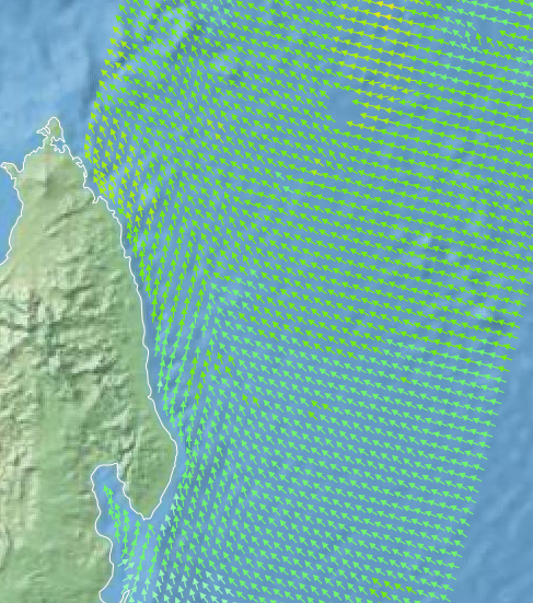
Products
ASCAT can produce wind vector maps. SatDump can't yet produce these products, but it will in the near future.
Conclusion
This concludes our overview of the instruments present on board polar orbiting satellites. As you have seen, it is quite easy to start developing your meteorologist's skills using the data received from the satellites. With some practice, you'll likely notice that the results can match and sometimes even exceed those of the usual weather apps!
Appendix
Weather forecasting example (APT data)
Here is an example on how to forecast weather for Genova, Italy using only data from APT broadcasts.
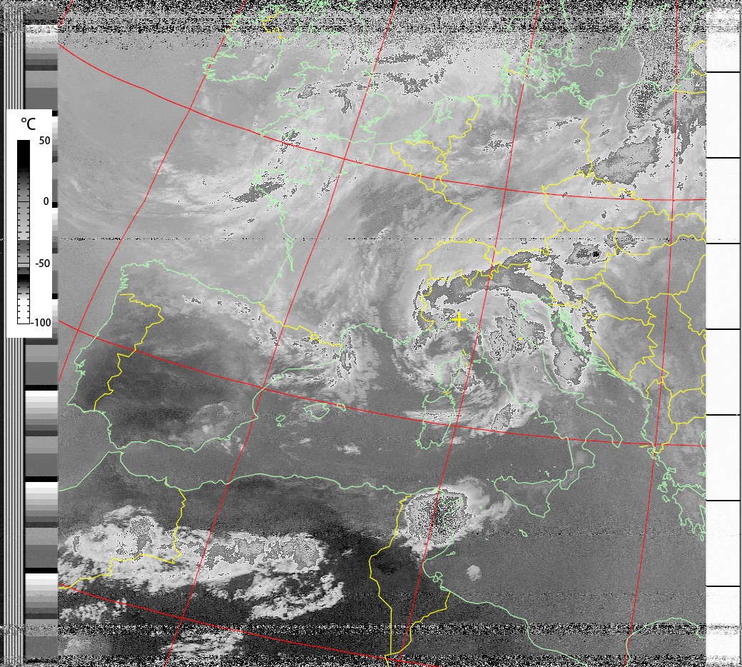
We have first received a NOAA 15 APT image which we have decoded with the Enhanced IR composite. The first thing we need to do is annotate the fronts and, if we can find them, low pressure areas.
In that case, we have an occluded front originating from a low pressure cyclonic area, that we can fairly easily find in the Atlantic.
We know this is an occluded front rather than a continuing cold front because we can find the depression area with clouds circling around it in a spiral fashion, and from the theory we know that in the mid-latitudes occluded fronts tend to form around these conditions.
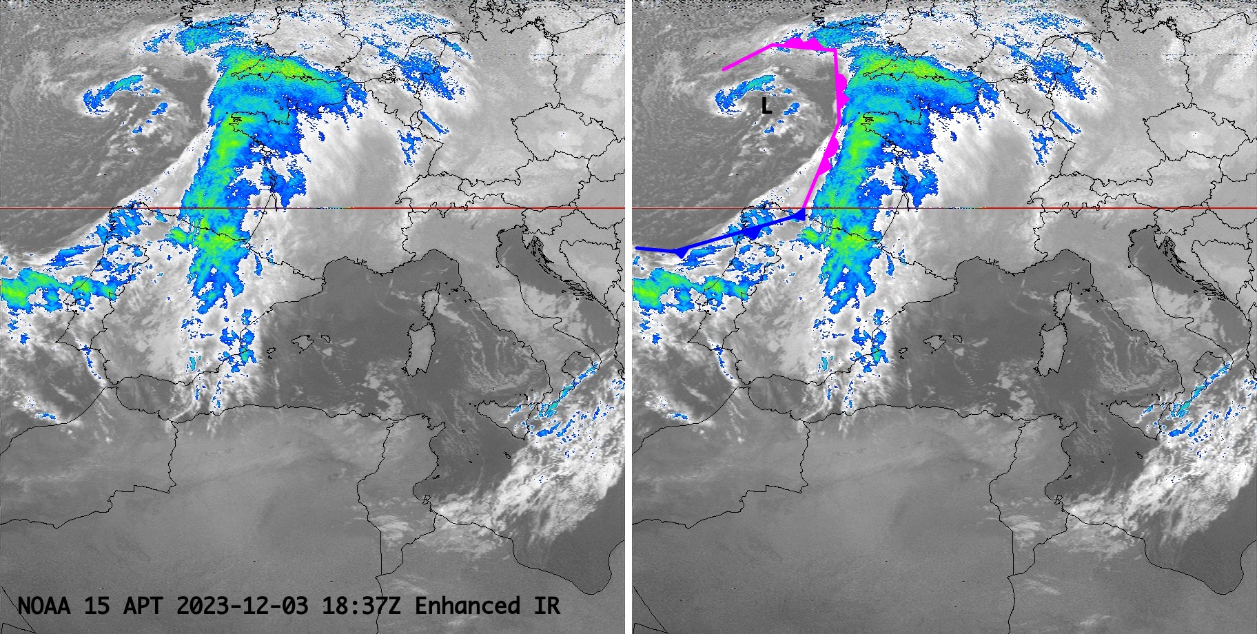 NOAA 15 Enhanced IR and annotated with fronts
We can fairly easily detect the direction of movement of the frontal system because we know that due to the Coriolis effect the systems (as a whole) travel from West to East.
We can also judge the estimated strength of the storm based on the cloud top temperature, in that case the cloud tops in the occluded front area have a temperature of around -50°C.
This means the storm is already well developed and it will likely rain, and snow above a certain altitude (we can determine it using the soil temperature, but this is beyond the scope of this example). Additionally we know that thunderstorms in this particular season are rare, therefore we expect no thunderstorm activity.
The next step is to predict how much time we have until the storm hits us. For that we use another satellite, the NOAA 19, and we check how much the storm has moved in that timeframe.
For that, we use a GCP (Ground Control Point) that we define arbitrarily. It must be easily recognizable and on the path of the storm. For this example, I've chosen the small state of Andorra as the first GCP, and the Gironde estuary near Bordeaux as the second.
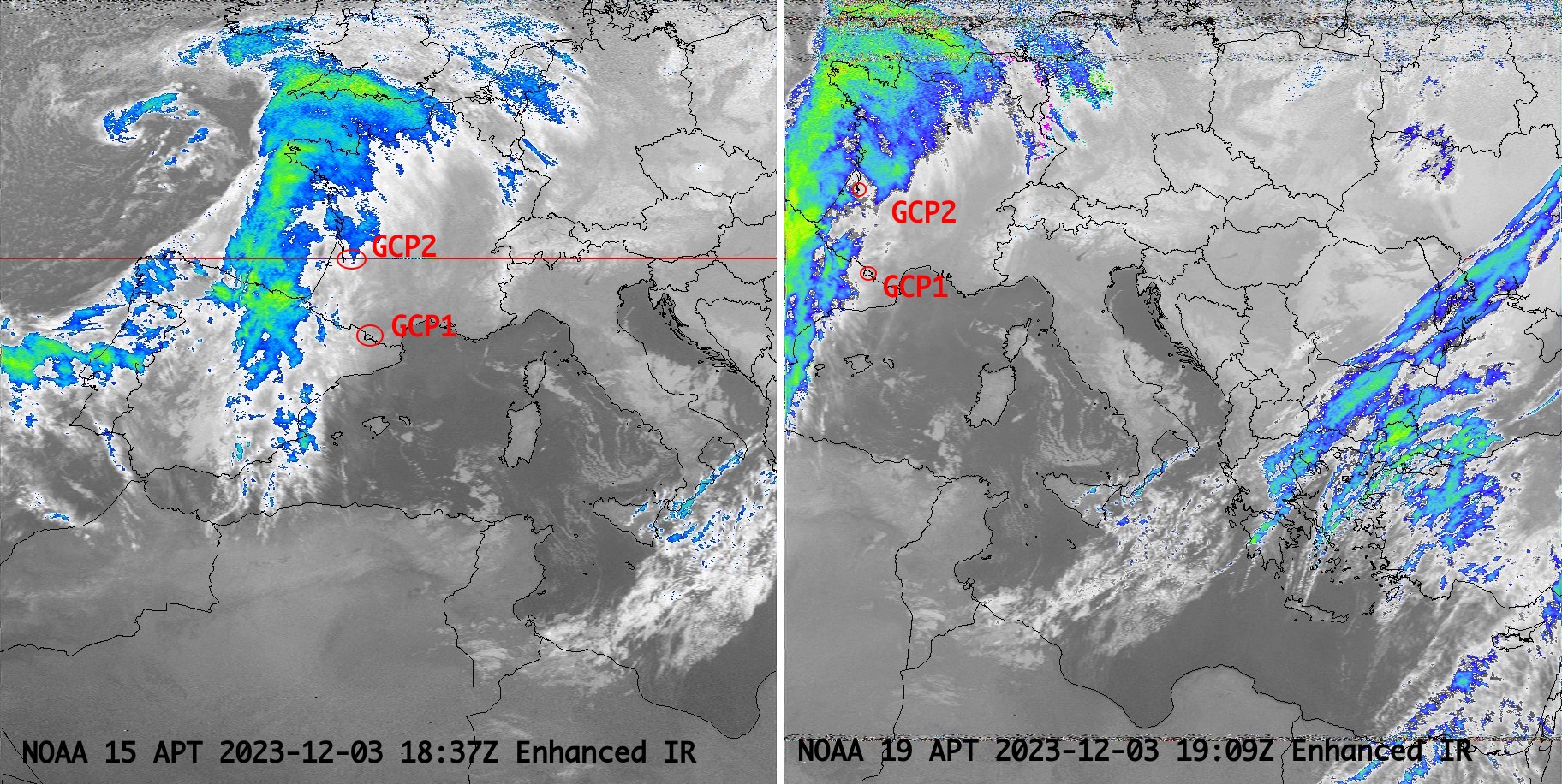 NOAA 15 and NOAA 19 Enhanced IR with Andorra and Bordeaux as GCPs
We can clearly see that the storm has moved quite a lot in just 32 minutes, especially the part near Andorra. We can therefore predict a time-of-arrival of about 5 hours (which means it will start raining at about 00:30Z).
Because we know that between Genova and the storm there are the Alps that oppose some resistance to its passage, we add half an hour to be safe, so we expect rain to happen around 01:00Z.
Additionally, we can estimate the time of passage (i.e. when the storm will clear us). Given the storm moves as a compact mass, we simply add the width of the frontal system to our calculation and we find that it will likely clear us in the afternoon around 11:00Z.
However, we know that Genova is a gulf surrounded on three sides by mountains (the Appennine chain) and this will cause more rain and a longer dwell time because of orographically induced precipitation. Adding an extra hour or two is a good idea.
If we'd like additional confirmation of our predictions, we can wait for a NOAA 18 pass and check if the rate of speed is still constant.
The last observation we can make is that behind our frontal systerm we have fairly clean skies, however there is a significant presence of altocumulus clouds. This is important as these clouds signify instability in the upper atmosphere and the probable arrival of another frontal system likely around December 6th.
Concluding, this is the weather report that we produced so far using two APT images:
Dec 04, morning
🌧️Dec 04, afternoon
🌧️Dec 04, evening
🌙Dec 05, morning
☀️Dec 05, afternoon
☀️Dec 05, evening
🌙Here is an image from NOAA 18 in both MCIR and MSA enhancements taken the next day, looks like our guess was correct!
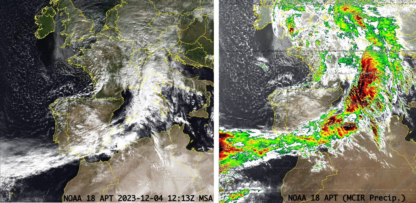 NOAA 18, note the fully developed frontal system over Genova that is soaking us with rain, as well as extended instability over the Atlantic materialized by a large presence of altocumuli
An additional reception of a NOAA 15 during the evening confirms that the storm has cleared us exactly on time and indeed tomorrow will be a beautiful day!
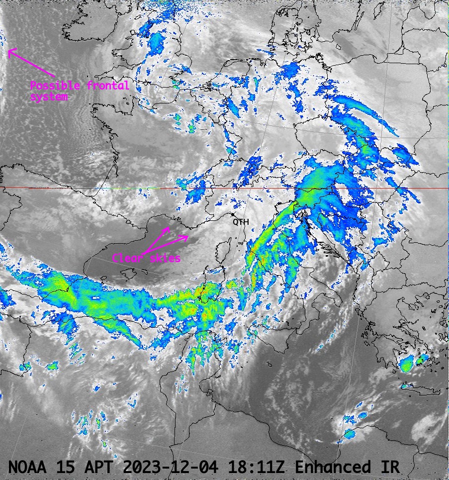 Confirmation of sunshine for tomorrow. Note the highlighted feature: it deserves further observation as it could very well be the next frontal system that could bring us rain again
Of course, each subsequent observation offers the opportunity of refining your model and predictions. This concludes our example!
Weather forecasting example (HRPT data)
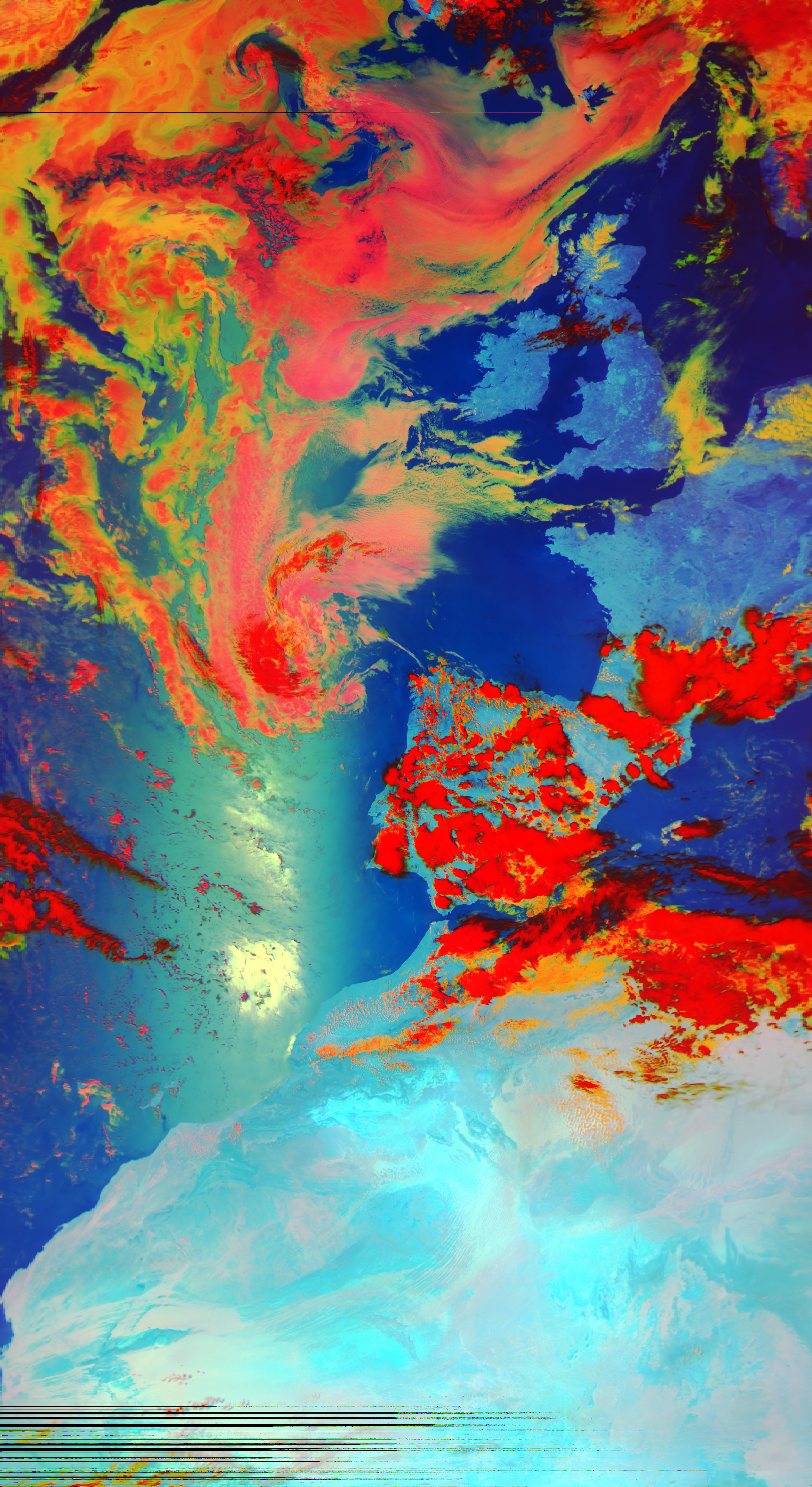
Again, we'll predict the weather in Genova, Italy as in the previous example. We start with a capture of NOAA 18 using two enhancements, visible and enhanced IR.
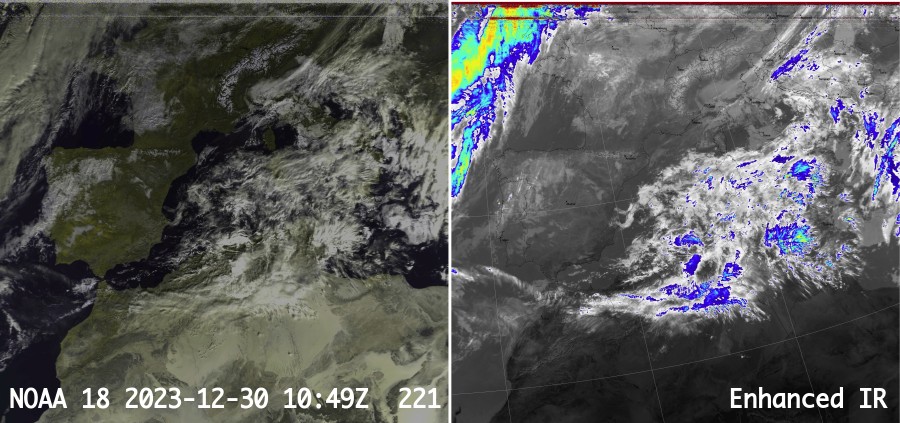 General view in Enhanced IR and 221 visible, from NOAA 18.
We should immediately recognize the incoming cold front over the Atlantic, so we know to expect it in a day or so, but what is happening right now over Northern Italy should be analyzed better.
First of all, using Day Microphysics we determine the kind of clouds over Pianura Padana. This is important, as if they're fog or low stratus clouds, it means there is a significant high pressure area, which could affect the arrival of the cold front.
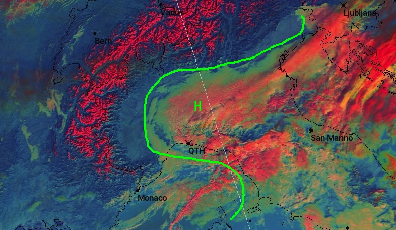
Day Microphysics reveals that the majority of clouds are low lying stratus clouds. The clouds over Toscana, on the other hands, are nimbostratus clouds that are precipitating thanks to orogenically induced precipitation over the Appennini and Alpi Apuane ranges.
With that in mind, we can say already that for the rest of the day there will be a low risk of some light to moderate rain drizzles over Genova immediately, with a more positive afternoon that will mostly be cloudy but with no rain. The evening will also be cloudy, with no risk of rain but lots of humidity.
A subsequent check of Meteor-M N°2-2 in the afternoon allows to check the progression of the cold front as we did with APT.
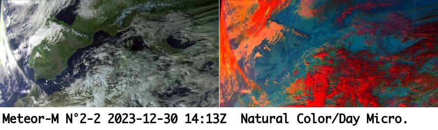
The front has reached A Coruña on the northern coast of Spain, about 200km in 3 hours.
Given the current rate of advance it is expected to arrive at our location in the late morning of December 31st.
Before we make predictions for New Year's Eve, we still need however to determine the entity of the incoming front, to see how much dwell time is expected. For that, we use NOAA 15 and 19, which enables us to do a further check on the rate of advance.
NOTE: This is not usually required if you have good reception. At my location, however, the reception to the North is severely limited by a mountain (Monte Cornua complex).
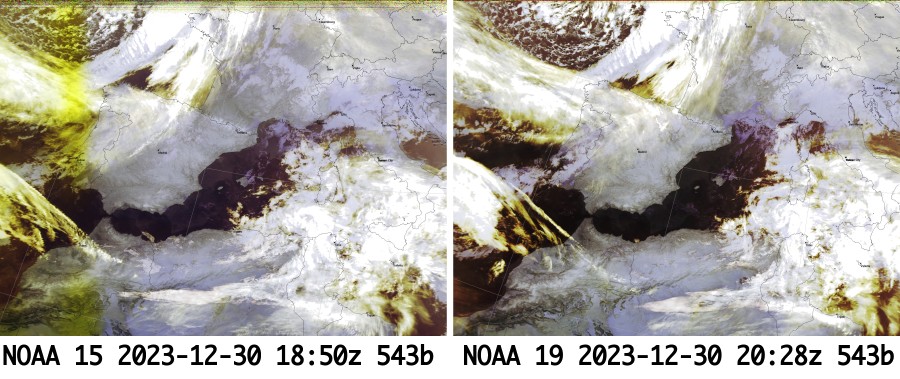
NOAA 15 and 19 show that the rate of advance is mostly unchanged.
Here is the weather report. Unfortunately, it looks like our New Year's Eve will be spoiled by rain :(
Dec 31, morning
🌧️Dec 31, afternoon
🌧️Dec 31, evening
🌧️Jan 01, morning
☁️Jan 01, afternoon
⛅Jan 01, evening
🌙[To be continued]
Version: v2.2.5